I wanted to setup google analytics for my octopress blog hosted on github pages. My situation was a little different than some of the existing tutorials because I’m using a custom domain, not the standard username.github.io domain. To get everything setup and working I did the following:

1. Create a Google Analytics account.
2. Tell your analytics account to monitor your custom domain. For me this was my www.mattnedrich.com domain, not the mattnedrich.github.io one.
3. Update your Octopress _config.yml file to include your analytics tracking id by setting the google_analytics_tracking_id: property. This tracking id will look something like UA-23414877-5
4. Generate and deploy your site

There are several posts online that talk about modifying the google_analytics.html octopress file. If you are using a custom domain with your github page you don’t have to do this (or at least I didn’t have to).

I wanted to manage my octopress blog from different computers. I have my blog source on github, so I thought it would be as easy as pulling it, making changes, generating, and deploying. However, I ran into several nuanced issues along the way which resulted in this error when I tried to deploy:

## Pushing generated _deploy website
To http://github.com/mattnedrich/mattnedrich.github.io
 ! [rejected]        master -> master (non-fast-forward)
error: failed to push some refs to 'http://github.com/mattnedrich/mattnedrich.github.io'
hint: Updates were rejected because the tip of your current branch is behind
hint: its remote counterpart. Integrate the remote changes (e.g.
hint: 'git pull ...') before pushing again.
hint: See the 'Note about fast-forwards' in 'git push --help' for details.

After being confused for a while, I came across this post and was able to successfully pull, modify, and deploy my blog from a second local repository. The only change I had to make from the instructions in the post was that I had to clone the master branch into the _deploy directory after running rake setup_github_pages as pointed out in the comments.

I have written an implementation of quicksort in C#. It can be found here.
https://github.com/mattnedrich/algorithms/blob/master/csharp/sorting/quicksort/Quicksorter.cs

It operates on anything that implements IComparable<T>. Suppose you have a class SortableObject that implements IComparable<SortableObject>. The usage model in this scenario would be

List<SortableObject> items = ...
Quicksorter<SortableObject> sorter = new Quicksorter<SortableObject>();
sorter.Sort(items);

My implementation contains a main Partition method that is called recursively to perform the sorting. In addition, there are two helper methods. The first, ChoosePivotIndex is responsible for choosing a pivot element from a list to be sorted. The current implementation naively selects a pivot at random. This method is virtual to keep it Open/Closed and allow others to extend it with a better pivot selection method if desired. The other method, Swap, swaps two elements in a list. I’ve found that in-lining the swapping yields faster performance, though I decided not to do so for clarity.

I benchmarked my implementation on different types of input of varying length. Results below.

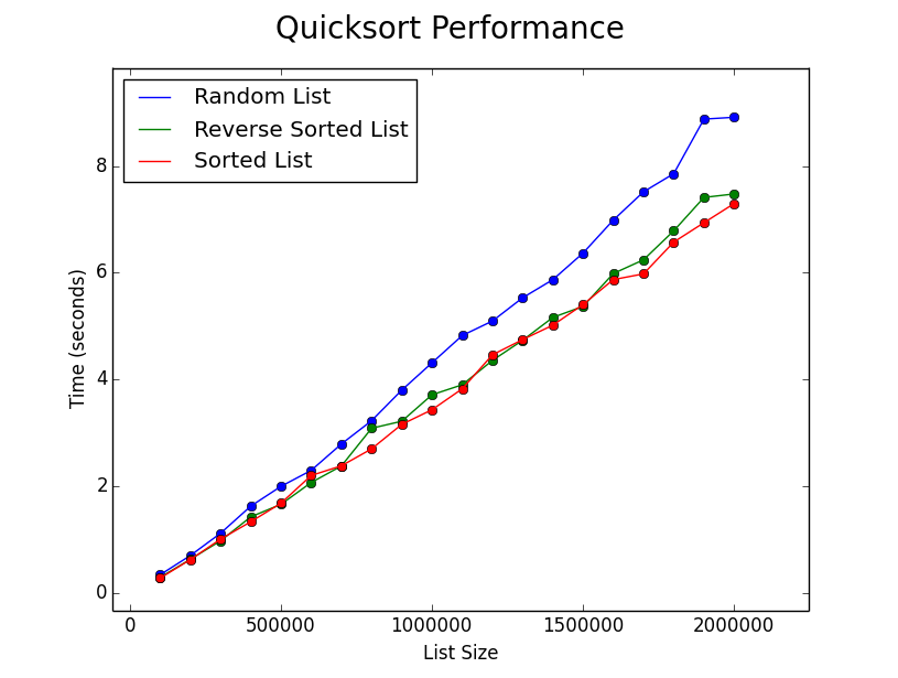
As displayed, my implementation (even with the naive pivot selection) is fairly robust to random, sorted, and reverse sorted lists.

I was having some fun implementing sorting algorithms and thought it might be interesting to compare my implementations against the C# built in List<T>.Sort. That was where the rabbit hole started.

Slow Quicksort

After finishing an implementation of quicksort I decided to give it a try on some big input. I wrote something to generate integer lists of arbitrary size with uniformly random elements. I ran some benchmarks, and then ran the same input against List<T>.Sort. My implementation was about ten times slower than the built in sort. I thought I must be doing something wrong. There must be some bug in my code. After all, the description of List<T>.Sort states that (from here)

• If the partition size is fewer than 16 elements, it uses an insertion sort algorithm.
• If the number of partitions exceeds 2 * LogN, where N is the range of the input array, it uses a Heapsort algorithm.
• Otherwise, it uses a Quicksort algorithm.

So the built-in sorting should be using Quicksort most of the time. I thought my implementation might just be slow, so I started to make some optimizations. My base implementation can be found here:
https://github.com/mattnedrich/algorithms/blob/master/csharp/sorting/quicksort/Quicksorter.cs

First I tried to in-line all of the function calls (e.g., ChoosePivotIndex and Swap). This yielded some performance improvement (about 10%). Next I played around with the pivot selection method. I was using a naive random pivot selection so I tried a median of three approach. This actually didn’t do much, though I suspect it is because my input was uniformly random. I tried parallelizing the calls to Partition. This actually slowed things down (probably due to the overhead of thread creation). Lastly, I cheated a bit and switched to insertion sort for small inputs, as the library sort does. This yielded the latest performance gain of around 20%. However, after all of my optimization, I was still around eight times slower than List<T>.Sort.

I was stuck, so I posted this, and learned that the .NET Framework special cases the sorting of built-in types (ints, string, etc). Just how much of a performance gain is achieved by doing this? I wanted to find out so I set up yet another experiment.

Int vs. IntInWrapper

I compared the performance of List<T>.Sort when using plain ol’ int’s to the performance when using int’s in a wrapper class. For the wrapper class I used:

public class IntInWrapper : IComparable<IntInWrapper>
{
    public int Val { get; set; }
    public IntInWrapper(int val)
    {
        Val = val;
    }

    public int CompareTo(IntInWrapper other)
    {
        if (this.Val < other.Val)
            return -1;
        else if (this.Val == other.Val)
            return 0;
        else
            return 1;
    }
}

I benchmarked sorting Lists of various sizes for the two input classes. Results are shown below. For each List size, sorting was performed ten times (each time on a different randomized list), and the average execution time was kept.

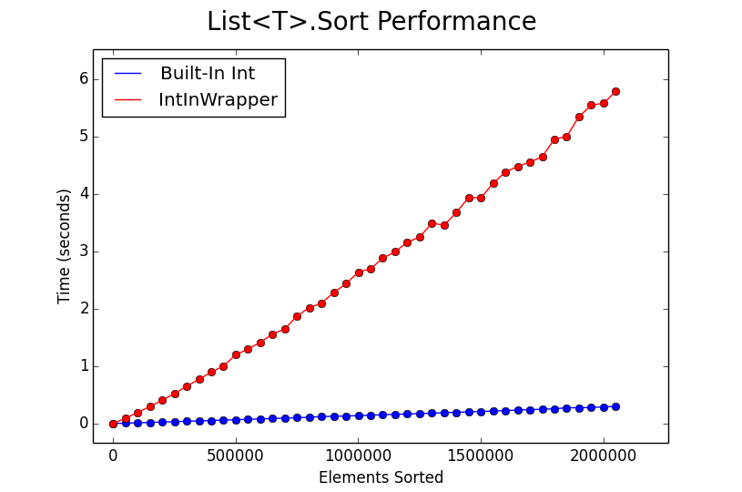
Sorting on wrapped int’s drastically degrades performance compared to plain int’s. From my understanding, this is largely due to the IComparable<T>.CompareTo function pointer being used for element comparison, rather than a simple > or < (which likely trickles down to a single assembly instruction). Anyway, the key learning from this is that use built-in types when you need sorting performance and be aware of the penalty associated with using custom types!

I often open command windows on Windows via shift + right click on a directory. It’s a handy way to open a cmd window right where you want one. Ironically the option directly below Open command window here is Open as Notebook in OneNote. I accidentally clicked the OneNote option and it turned out to be a pretty interesting 10 pixel mistake.

Some backstory - my original intent was to open a cmd window to the source directory of my blog to build it (I’m using Octopress). At first it wasn’t clear what clicking the OneNote option actually did. However, after a little poking around I was seeing a OneNote Table Of Content.onetoc2 file in every directory of my blog output. That is, I didn’t see these in the blog source directory, but every time I would build my blog they would show up in every output directory.

I tried grepping for interesting files/directories in the blog source, but nothing showed up. I tried manually browsing through the source directory structure. Also note that I had show hidden files and folders turned on. Still, I found nothing.

After some digging, and a lot of help from this post it turns out that there were several OneNote files embedded and hidden in every directory of my blog source. The only way I was able to see them was to display them in a cmd window via

dir /A:H /B

After it was clear that they were indeed there but hidden, I was able to delete them via

del /S /A:H *.onetoc2

I’ve written a general K-Means implementation in Python. It can be found here:
https://github.com/mattnedrich/algorithms/blob/master/python/clustering/kmeans/kmeans.py

Everything is contained in one file, kmeans.py The usage model is the following

import kmeans

# observations
#  - list of items to be clustered
# numMeans
#  - number of clusters desired
# featureVectorFunc
#  - function that extracts a feature vector (in the form of a Tuple) from an observation
# maxIterations
#  - optional param, can be used to set a max number of iterations
[clusters, error, numIter] = kmeans.cluster(observations, numMeans, featureVectorFunc, maxIterations)

My goal was to make something simple and accessible that doesn’t require additional libraries (e.g., numpy is not required). The user must do one thing - provide a featureVectorFunc that takes in an observation from the input, and returns a feature vector in the form of a Tuple. This function would look something like this:

def someFeatureVectorFunc(obs):
    featureVectorAsTuple = extractFeatureVector(obs)
    return featureVectorAsTuple

The output clusters is a list of cluster objects. Each cluster has a field called observations. This is subset of the original input observations (stored in a list).

Example Results

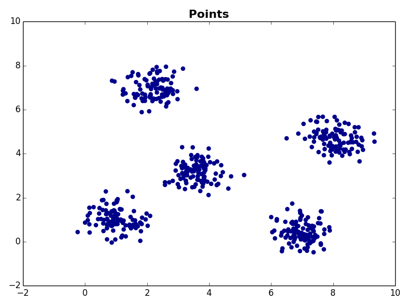
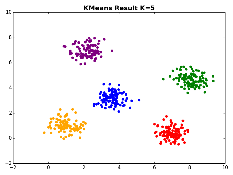
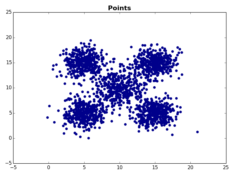
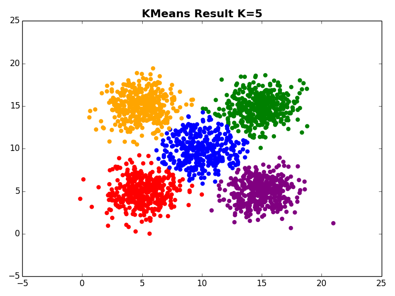
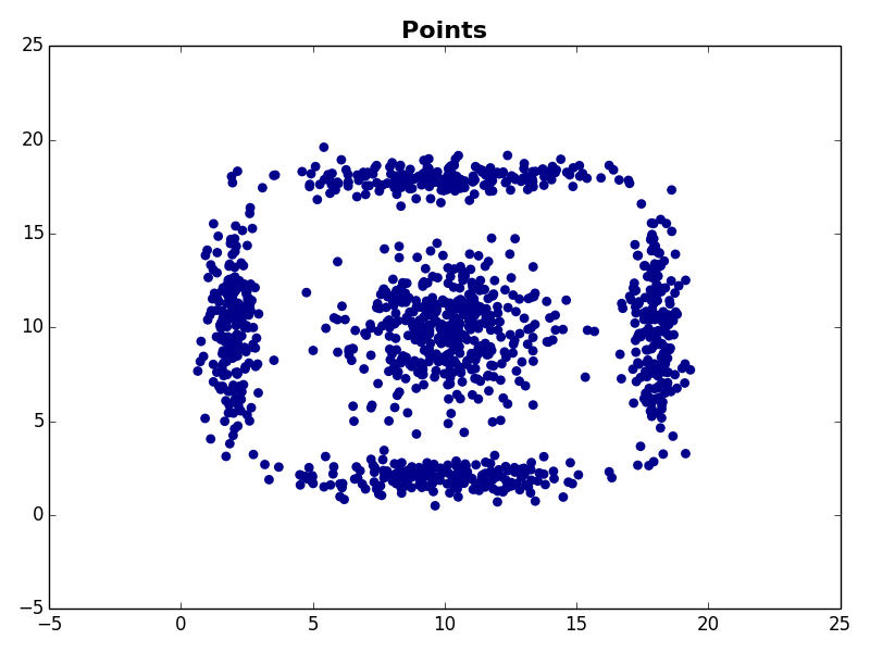
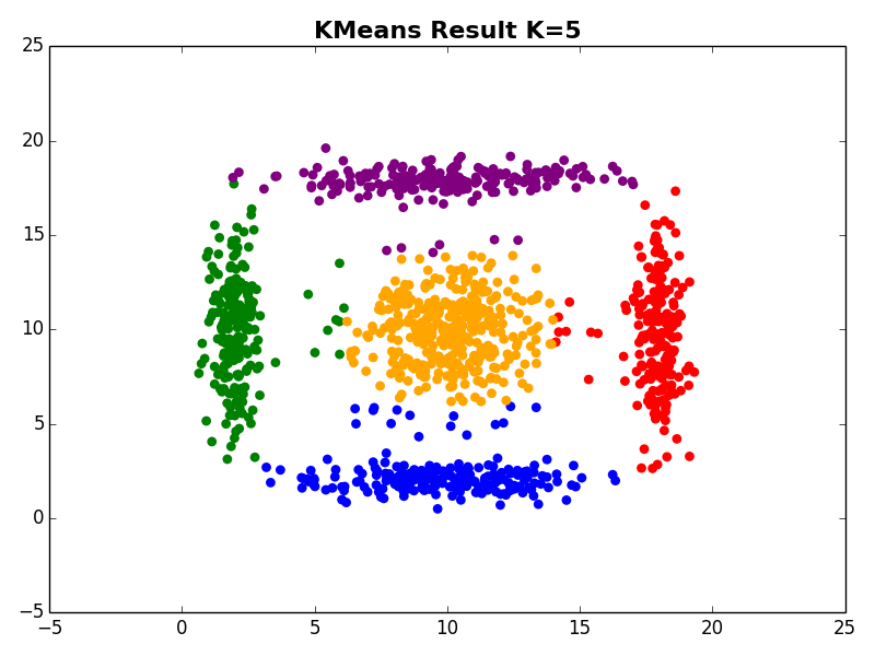
I ran my implementation on the three synthetic datasets below. For each dataset, I used K=5. I also ran K-Means 10 times and selected the result with the lowest error.

Dataset 1

Dataset 2

Dataset 3

I occasionally need to benchmark some code. In C#, this can easily be done using the Stopwatch class. After writing the same boilerplate Stopwatch wrapper enough times I decided to throw together a simple Benchmarker class.

public static class Benchmarker
{
    public static TimeSpan RunOnce(Action action)
    {
        Stopwatch stopwatch = Stopwatch.StartNew();
        action();
        stopwatch.Stop();
        return stopwatch.Elapsed;
    }
    
    public static IEnumerable<TimeSpan> RunMany(Action action, int runCount)
    {
        List<TimeSpan> results = new List<TimeSpan>();
        for (int i = 0; i < runCount; i++)
            results.Add(RunOnce(action));
        return results;
    }
}

This allows any code to be easily called and timed. For example, suppose you have a void Method called Foo. This can be timed via:

TimeSpan timespan = Benchmarker.RunOnce(() => Foo());

Similarly, if you want to benchmark a method that happens to return something like this

int bar = FooWithReturnValue();

you can use the above Benchmarker class via

int bar;
TimeSpan timespan = Benchmarker.RunOnce(() => bar = FooWithReturnValue());

I’ve put this on github: https://github.com/mattnedrich/tools/tree/master/csharp/Benchmarker.cs

I’ve dabbled in Android development in the past, but haven’t done much with emulation. In my experience the Android emulators are too slow to use, and I’ve usually used my phone for testing/debugging.

Intel’s Hardware Accelerated Execution Manager (HAXM) uses CPU virtualization to speed up Android emulators. I wanted to give it a try.

CPU Compatibility

I have a pretty old desktop machine, so I wasn’t even sure if my CPU supported hardware virtualization. Poking around a bit, there are a few Windows utilities that can be used to determine if virtualizaiton is enabled on your CPU.

• http://www.intel.com/support/processors/sb/cs-030729.htm
• http://www.microsoft.com/en-us/download/details.aspx?id=592
• https://www.grc.com/securable.htm

The Intel utility looks like this:

Results

With virtualization verified and enabled, I followed this writeup to install everything and setup an x86 Android emulator.

So how did it work? It wasn’t that much faster, but there was a noticeable difference. The HAXM emulator booted in 182 seconds, compared to 282 seconds for the ARM emulator. With both emulators open, I could click on a button (e.g., open the Settings app) and the HAXM emulator would finish first, usually by 1-5 seconds depending on the task. As a disclaimer, I was using a pretty old computer. I’m not sure what impact that had on my experience.

Regardless, while there was some speedup, it’s nowhere close to testing/debugging on a real phone (as is to be expected). The emulator is nice for testing different phones/configurations, but in general I find it much nicer to just push my application to a real phone.

What is K-Means

Need to cluster some data? K-Means is one of the most common and simplistic clustering algorithms. It works by partitioning a data set into K different groups (clusters). In this post, we’ll walk through the basics of K-Means, explain how it works, and touch on some of its strengths and weaknesses.

The Input

The input to K-Means is a set of data and a parameter K, which defines the number of clusters to partition the data into. Each input observation is a vector in d-dimensional space. The number of dimensions doesn’t matter.

The Algorithm

The goal of the K-Means algorithm is to find a partitioning of the input data that minimizes within-cluster sum of squares (WCSS). Simply put, the goal is to find a clustering such that the points in each cluster are close together. This objective function (we’ll call it $J$) can be expressed as:

Here, $K$ is the number of clusters, $N$ is the number of points, $\mu_k$ is the cluster centroid for cluster $k$, and $x_i$ corresponds to input observation $i$. Informally, this function computes the variance of the observations around each cluster centroid (for a given set of K centroids). The goal is the minimize this function. Each iteration of the K-Means algorithm reduces the objective function, moving closer to a minimum.

K-Means uses an Expectation Maximization approach to partition the input data and minimize the WCSS. Conceptually, we start with an initial set of cluster centroids (with an implicitly defined WCSS score). The goal is to figure out how to move these centroids around to make the WCSS score as small as possible. The algorithm can be expressed as

1. Initialize cluster centroids
while not converged:
    2. Cluster Assignment - assign each observation to the nearest cluster centroid
    3. Update Centroids - update the cluster centroid locations

Let’s go over each of these steps.

1. Initialize Cluter Centroids

The first step is to choose an initial set of K cluster centroid locations. This can be done many ways. One approach is to choose K random locations in whatever dimensional space you’re working in. This approach may work, but in practice it may be difficult to choose these locations well. For example, it’s undesirable to choose locations very far away from any of the data. Another, perhaps better, approach is to choose K random observations from the input dataset.

2. Cluster Assignment

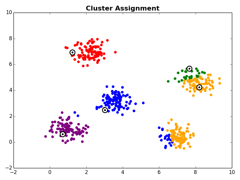
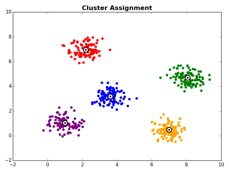
In the cluster assignment step each observation in the dataset is assigned to a cluster centroid. This is done by assigning each observation to it’s nearest centroid.

3. Cluster Centroid Update

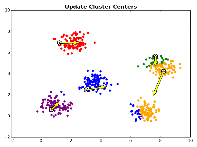
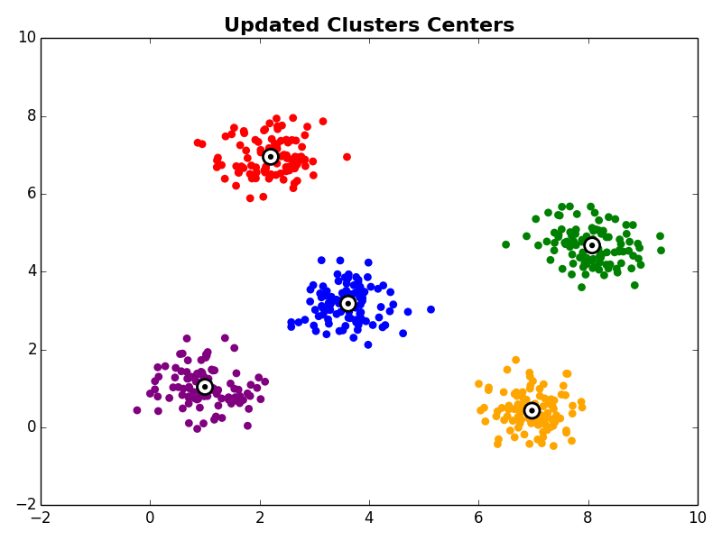
Next, in the cluster centroid update step, each cluster centroid is updated to be the center (e.g., mean) of the observations assigned to it.

Steps 2 and 3 are repeated until the algorithm converges. There are a few commonly used ways to determine convergence.

1. Fixed Iteration Number - K-Means can be terminated after running for a fixed number of iterations. Obviously, this approach does not guarantee that the algorithm has converged, but can be useful when an approximate solution is sufficient, or termination is difficult to detect.
2. No Cluster Assignment Changes - This is the most common approach. If no observations change cluster membership between iterations, this indicates that the algorithm will not continue further, and can be terminated.
3. Error Threshold - An error threshold can also be used to terminate the algorithm. However, choosing a good threshold is problem and domain specific (e.g., a threshold that works well for one application may not work well for another).

Example

K-Means is often best understood visually, so let’s walk through an example. Suppose you have the following data in two dimensional space.

The first step is to choose K starting cluster centers. For our example we will set K=5. For our example we’ll randomly select five observations from our data set to be the initial cluster centroids:

With the initial cluster centroids selected, steps 2 and 3 are iterated as described above.

Other Comments

Repeated Runs

It’s very important to note that K-Means is notorious for getting stuck in local minima. This means that there is no guarantee that running K-Means will actually find the optimal solution for a given starting point (set of initial cluster centroids). To overcome this, K-Means is often run multiple times with different initial cluster centroids, and the clustering with the lowest error (WCSS) is chosen.

Choosing K

This video from Andrew Ng’s Machine Learning course on Coursera does a great job summarizing the task of choosing K. In general, there is no great general purpose method. Choosing K often requires manual input based on data visualizaiton or other domain knowledge. Interestingly, for some applications, K may already be known. The T-Shirt sizing example in the video is a great example of this. For these types of problems the goal is to partition the data into a pre-defined number of sets, rather than learning how many distinct sub-sets make up the original input data.

Strengths and Weaknesses

Strengths: K-Means is great because it’s simple and fast. There are several off the shelf implementations available on the internet, and if they’re not good enough, it’s not terribly difficult to implement K-Means on your own.
Weaknesses:The main weakness of K-Means is that it doesn’t work that well for non-spherical clusters. Also, as we discussed earlier, it’s also notorius for getting stuck in local minima, and requires the user to choose K.

I found this post helpful when trying to enable LaTeX style math formulas in Octopress:

http://blog.zhengdong.me/2012/12/19/latex-math-in-octopress

It’s also worth noting that when you change Octopress themes source/_includes/custom/head.html seems to get overwritten, so you have to re-add the provided snippet.